Tutorial
Imports
import numpy as np
import h5py
import glob
from astropy import units as u
from astropy.constants import k_B, m_p,m_e, sigma_T, c
import re
import matplotlib.pyplot as plt
import warnings
warnings.filterwarnings("ignore")

def sort_nicely(l):
    """ Sort the given list in the way that humans expect.
    """
    convert = lambda text: int(text) if text.isdigit() else text
    alphanum_key = lambda key: [ convert(c) for c in re.split('([0-9]+)', key) ]
    l.sort( key=alphanum_key )
How to use the zooms
Welcome to CAMELS-zoomGZ! This suite of simulations is unique in that it only contains zoom-in simulations. Here are some key details:
Each zoom has at least 1 “pure” halo: purity is where low resolution dark matter mass is less than 5% of total mass
Halos span a range of \(10^{13}M_\odot\leq M\leq 10^{14.5}M_\odot\)
The semi-complete 28 dimensional TNG astrophysical + cosmological parameter space is spanned for each zoom
Resolution matches CAMELS boxes in zoom-in region (About TNG300-1)
Each zoom lives in a 200 Mpc/h parent box
Each zoom has a DMO counterpart
Initial conditions were chosen following CARPoolGP setup: half of the sims are surrogate simulations (more on this below)
Because of CARPoolGP we can emulate halo quantities throughout the entire parameter space
This tutorial will introduce tools for using the simulations, so that you can utilize them for whatever scenario you are interested in! I do not include (yet) CARPoolGP tutorial, but hopefully this will help you get started messing around with the zooms. Note that they are not all complete/on the same super computer! so this will be somewhat updated soon
Reading in zoom-in information
Halo properties
The zooms are run with arepo, and follow very similarly to the CAMELS/Illustris/TNG format. The only difference is that there is an additional particle type for low-resolution DM particles:
PartType0 = Gas
PartType1 = High res DM
PartType2 = Low res DM
PartType3 = Tracers
PartType4 = Stars
PartType5 = Black holes
So to find the zoom-in halo, look for the most massive halo with the smallest amount of contamination
def pick_halo(contamination, level=0.05):
    """
    Choose the largest fof halo with the smallest contamination

    Parameters
    contamination: ratio of low resolution to high resolution dm for all fof halos
    level: percent level of contamination default is 5%

    returns
    halo_n: halo index of zoom-in halo
    """
    try:
        if len(contamination)==1:
            halo_n = 0
        else:
            contamination = contamination < level
            indices = np.arange(len(contamination))
            halo_n = indices[contamination][0]

    except IndexError:
        # Some zooms simply have the zoom-in halo as the only large halo
        halo_n = 0
    return halo_n, contamination[halo_n]


def FOF_properties(zoompath, fields, snapNum=90, level=0.05, hydro=True,
                   return_contamination=False, return_offsets=False):
    """
    extract FOF properties of the zoom-in halo

    Parameters
    halopath: path to the directory of fof files for a zoom
    fields:   fof fields to extract
    snapNum:  snapshot corresponding to redshift/scale factor (default z=0)
    level:    level of contamination to determine zoom in halo (default 5%)
    hydro:    boolean where true is hydro false is dmo
    return_contamination: if interested in contamination level of halo
    return_offsets: if interested in particles from halo

    Returns
    field_dict: Dictionary of desired fields
    """
    fields = np.atleast_1d(fields)
    if hydro:
        sim_type='Hydro'
    else:
        sim_type='DMO'

    halopath =  '%s/%s/groups_%s/fof_subhalo_tab_%s.0.hdf5'%(zoompath,
                                                             sim_type,
                                                           str(snapNum).zfill(3),
                                                           str(snapNum).zfill(3))

    field_dict = {}
    with h5py.File(halopath, 'r') as f1:

        # Find the halo of interest by checking purity
        masses = f1['Group/GroupMassType'][:]*1e10
        contamination = (masses[:, 2] / masses[:, 1])
        halo_n, halo_contamination = pick_halo(contamination)
        field_dict['FOF_ID'] = halo_n

        if return_contamination:
            field_dict['contamination'] = halo_contamination

        # Halo Quantities
        for field in fields:
            field_dict[field] = f1['Group/%s'%field][halo_n]

        if return_offsets:
            group_len = f1['Group/GroupLenType'][:]
            offsets   = [np.sum(group_len[:i], axis=0) for i in range(halo_n+1)]
            field_dict['offset'] = offsets

    return field_dict
You can input any field from the list of fields (see TNG documentation or CAMELS documentation)
For example we can extract the halo mass, radius, and center of mass for one of the zooms like so:
# Change this to the location where the simulations are in binder or local
basepath = '/mnt/home/mlee1/Sims/IllustrisTNG_zoom/'

# Pick a zoom always zoom_#
zoom_no = 0
zoompath = basepath + 'zoom_%i'%zoom_no

# Pick a redshift (via snapshots) and if hydro or DMO (boolean for hydro)
snapNum=90
hydro=True

#choose your favorite fields
fields = ['Group_M_Crit200', 'Group_R_Crit200', 'GroupPos', 'GroupLenType']

# extract properties
FOF = FOF_properties(zoompath, fields, snapNum=snapNum, hydro=hydro, return_contamination=True)

print('zoom_%i properties\n'%zoom_no)
for k,v in FOF.items():
    print(k+': ', v)
zoom_0 properties

FOF_ID:  0
contamination:  0.00037551197
Group_M_Crit200:  10399.345
Group_R_Crit200:  764.83
GroupPos:  [ 99021.41 102986.68  98816.51]
GroupLenType:  [1478429 2066512      97 1760141  264924      32]
Particle information
We can use the halo information to find the particle information. There are two approaches here, you can load in all particles chosen as part of the halo, or just particles within sphere of some radius definition. I will show both ways and compare ther results
def load_all_particles(zoompath, fields, parttype, snapNum=90, hydro=True, inds=None):
    """
    Extract all particle information from simulation for given fields

    Parameters
    zoompath: path to the zoom
    fields: fields to extract see TNG or CAMELS documentation
    parttype: int for the type of particle following arepo parttypes
    snapNum: int of snapshot
    hydro: if true, this is the hydro, if false, this is DMO
    inds:  particle indexes. If none, returns full snapshot

    Returns
    field_dict: dictionary of all fields
    """

    fields = np.atleast_1d(fields)
    if hydro:
        sim_type='Hydro'
    else:
        sim_type='DMO'
        assert parttype not in [0,4,5]

    snappath   = '%s/%s/snapdir_%s/'%(zoompath, sim_type, str(snapNum).zfill(3))
    snaps      = glob.glob(snappath+'*.hdf5')
    sort_nicely(snaps)
    parttype   = "PartType" + str(parttype)

    field_dict = {}
    for field in fields:
        store_field = []
        for snap in snaps:
            try:
                with h5py.File(snap, 'r') as fname:
                    store_field.append(fname[parttype+'/' + field][:])
            except KeyError:
                pass
        f = np.concatenate(store_field)
        if inds is None:
            field_dict[field] = f
        else:
            field_dict[field] = f[inds]
    return field_dict

def load_halo(zoompath, fields, parttype, snapNum=90, hydro=True, radius_def='Group_R_Crit200', spherical=True):
    """
    Extract all particle information from the zoom-in halo

    Parameters
    zoompath: path to the zoom
    fields: fields to extract see TNG or CAMELS documentation
    parttype: int for the type of particle following arepo parttypes
    snapNum: int of snapshot
    hydro: if true, this is the hydro, if false, this is DMO
    radius_def: If using radius to define the halo, pick the definition (500 vs 200), defaultsto R200
    spherical: boolean controling if halo is extracted using FOF particles or spherical inside R200

    Returns
    field_dict: dictionary of all fields for the zoom-in halo's particles
    """
    halo_fields = FOF_properties(zoompath, ['GroupPos', 'GroupLenType', radius_def], return_offsets=True)

    # For all fof particles in halo
    if not spherical:
        halo_n = halo_fields['FOF_ID']
        inds = np.arange(halo_fields['offset'][halo_n][parttype], halo_fields['GroupLenType'][parttype])
    else:
        particle_coords = load_all_particles(zoompath, 'Coordinates', parttype, snapNum=snapNum, hydro=hydro)
        inds   = np.sqrt(
                    np.sum(
                        (particle_coords['Coordinates']-halo_fields['GroupPos'])**2,
                    axis=-1)
                ) <= halo_fields[radius_def]
        del halo_fields

    field_dict = load_all_particles(zoompath, fields, parttype, snapNum=snapNum, hydro=hydro, inds=inds)
    return field_dict
def temperature(Xe, internal_e):
    """
    https://www.tng-project.org/data/docs/faq/#gen6
    """
    XH = 0.76
    mu = 4./(1.+3.*XH+4.*XH*Xe) * m_p
    Temp = 2./3. * internal_e * mu
    return (Temp/k_B).to(u.K)
Lets look at the gas coordinates, colorcoded by the temperature. For this we need coords, internal energy and electron abundance, which we can load for both the spherical and standard fof.
# Load in the required parameters
particles_spherical = load_halo(zoompath, ['Coordinates', 'InternalEnergy', 'ElectronAbundance'], 0)
particles_fof       = load_halo(zoompath, ['Coordinates', 'InternalEnergy', 'ElectronAbundance'], 0, spherical=False)
# Compute temp, note I am using astropy constants for ease
temp_spherical  = temperature(particles_spherical['ElectronAbundance'], particles_spherical['InternalEnergy'] * (u.km/u.s)**2  )
temp_fof        = temperature(particles_fof['ElectronAbundance'], particles_fof['InternalEnergy'] * (u.km/u.s)**2  )
# Plot the coordinates in XY with the temperature scaling the color
fig, axs = plt.subplots(ncols=2, figsize=(10, 4), sharex=True, sharey=True)
colormap = plt.cm.jet #or any other colormap
from matplotlib import colors
normalize = colors.Normalize(vmin=5, vmax=8)

im1 = axs[0].scatter(particles_spherical['Coordinates'][::10, 0]/1000, particles_spherical['Coordinates'][::10, 1]/1000,
               s=0.001, alpha=0.6, c=np.log10(temp_spherical[::10].value), cmap=colormap, norm=normalize)
im2 = axs[1].scatter(particles_fof['Coordinates'][::10, 0]/1000, particles_fof['Coordinates'][::10, 1]/1000,
               s=0.001, alpha=0.6, c=np.log10(temp_fof[::10].value), cmap=colormap, norm=normalize)

axs[0].set_xlabel('X [Mpc/h]')
axs[1].set_xlabel('X [Mpc/h]')
axs[0].set_ylabel('Y [Mpc/h]')

cb = fig.colorbar(im2, ax=[axs[0], axs[1]], orientation='vertical')
cb.set_label('Log(T)')
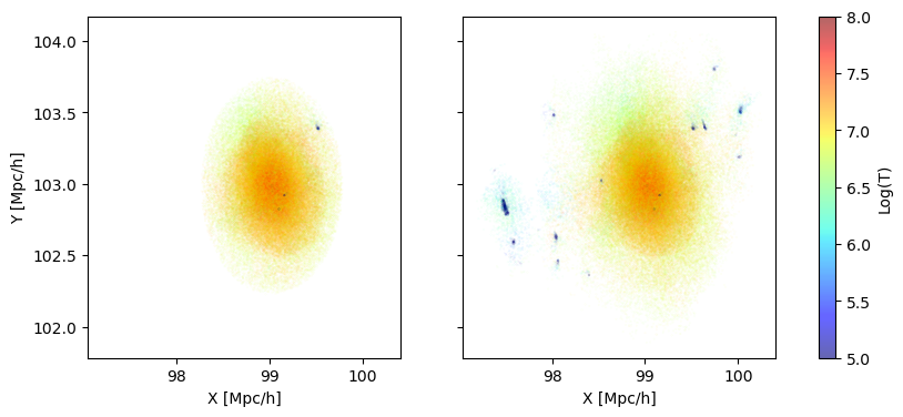
Notice that the halo is near 100-100. This is the center of the box, and means that we are indeed looking at the halo we intended to zoom in on.
You can extract any quantity or field in this way same way.
Parameter values
Each zoom is run with a different set of parameters. You can find these in the ‘PARAMS.txt’ file. The details of each parameter can be found in the param_info file from camels which includes the prior bounds and fiducial values.
There are other parameters in this file including the resolution, random seed, etc. So using the below you can find the cosmo, astrophysical, and mass parameters used.
One thing to note is that the mass parameter is NOT the true mass of the halo. It is the intended mass of the parent halo. This means that some zooms will have masses greater than, or less than the mass of the intended halo. Further, Surrogates are bijectively matched to base samples (see more of this in the CARPoolGP section). So they are the same halo but with different parameter values, which could lead to much greater or smaller masses than listed in the file.
import pandas as pd
params_path = 'GZ28_params.csv'
param_info = pd.read_csv('GZ28_param_minmax.csv', index_col=0)
param_info = pd.concat([param_info,
                        pd.DataFrame({'ParamName':'Mass', 'AbsMaxDiff':3.16-0.1, 'LogFlag':0, 'FiducialVal':1, 'MinVal':0.1, 'MaxVal': 3.16, 'Description':'Halo mass in units of 10^{14}M_sun'}, index=[0])]
                       , ignore_index=True)
This data frame param_info holds the names, priors, fiducial and
description
Now to actually extract the parameters, we open the file with all of the parameters and take out just the cosmological, astrophysical, and mass parameters used
params = pd.read_csv(params_path, index_col=0)
true_masses = []
for i in range(768):
    zoompath = basepath + '/zoom_%i'%i
    try:
        Mass = FOF_properties(zoompath, 'Group_M_Crit200')
        true_masses.append(Mass['Group_M_Crit200'])
    except:
        true_masses.append(0)

params['Mass'] = np.array(true_masses)*1e10 #put into solar masses
params['zoom_num'] = np.arange(768)
_ = plt.hist(np.log10(params['Mass']), edgecolor='k', bins=np.arange(10, 16, 0.33))
plt.xlabel('Log M')
plt.ylabel('N');

This might look strange, but this is primarily the effect of surrogates stretching or contracting the mass of the base halo. To show this, we can ID the surrogates knowing that the simulations were run with 3 batches:
128 base, 128 surrogate
128 base, 128 surrogate
64 base, 64 surrogate
64 base, 64 surrogate
Which are ordered in this exact way
fig, axs = plt.subplots(ncols=2, sharex=True, sharey=True, figsize=(8, 4))
_ = axs[0].hist(np.log10(params.loc[np.isnan(params['Surrogate']), 'Mass']), edgecolor='k', bins=np.arange(10, 16, 0.33))
_ = axs[1].hist(np.log10(params.loc[~np.isnan(params['Surrogate']), 'Mass']), edgecolor='k', bins=np.arange(10, 16, 0.33))
axs[0].set_title('Base Simulations')
axs[1].set_title('Surrogate Simulations')
axs[0].set_xlabel('Log M')
axs[1].set_xlabel('Log M')
axs[0].set_ylabel('N');

So you see that the Surrogates areoutside of the prior range, but this is ok. This is just an effect of having a surrogate simulation at a different location in parameter space for the same halo.
Ok, so what is a surrogate? It is a simulation of the exact same halo, but at a point in parameter space occupied by other surrogates… Which is not at the same location as the base!. So you can think of base simulations as sampling a large number of parameter space locations but are isolated, while surrogates sample a few locations in parameter space, but are grouped together at that location. Every base has a surrogate match, meaning that they were run with the same initial seed and chosen to be the same halo. Note that the parameter islands are for the astrophysical and cosmological parameters, as the mass parameter depends on the resulting halo.
So for example here is a base surrogate pair
# Load in the required parameters
base_halo = basepath + '/zoom_1'
particles_base  = load_halo(base_halo, ['Coordinates', 'InternalEnergy', 'ElectronAbundance'], 0, spherical=False)

surrogate_halo = basepath + '/zoom_129'
particles_surr = load_halo(surrogate_halo, ['Coordinates', 'InternalEnergy', 'ElectronAbundance'], 0, spherical=False)
# Compute temp, note I am using astropy constants for ease
temp_base      = temperature(particles_base['ElectronAbundance'], particles_base['InternalEnergy'] * (u.km/u.s)**2  )
temp_surr = temperature(particles_surr['ElectronAbundance'], particles_surr['InternalEnergy'] * (u.km/u.s)**2  )
# Plot the coordinates in XY with the temperature scaling the color
fig, axs = plt.subplots(ncols=2, figsize=(10, 4), sharex=True, sharey=True)
colormap = plt.cm.jet #or any other colormap
from matplotlib import colors
normalize = colors.Normalize(vmin=5, vmax=8)

im1 = axs[0].scatter(particles_base['Coordinates'][::10, 0]/1000, particles_base['Coordinates'][::10, 1]/1000,
               s=0.1, alpha=0.4, c=np.log10(temp_base[::10].value), cmap=colormap, norm=normalize)
im2 = axs[1].scatter(particles_surr['Coordinates'][::10, 0]/1000, particles_surr['Coordinates'][::10, 1]/1000,
               s=0.1, alpha=0.4, c=np.log10(temp_surr[::10].value), cmap=colormap, norm=normalize)

axs[0].set_xlabel('X [Mpc/h]')
axs[1].set_xlabel('X [Mpc/h]')
axs[0].set_ylabel('Y [Mpc/h]')

cb = fig.colorbar(im2, ax=[axs[0], axs[1]], orientation='vertical')
cb.set_label('Log(T)')
axs[0].set_title('Base halo')
axs[1].set_title('Surrogate halo');
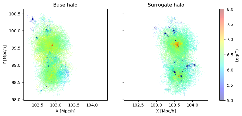
Notice how the surrogate halo is much smaller! But this makes sense, as the parameters themselves are different. particularly, look at \(\Omega_m\) and the mass of the resulting halos. The halos are the same (chosen by bijective matching), but because of the smaller matter density, the surrogate is less massive. Surrogates are chosen to live on a set of islands that are closest to their base, but because of the massive parameter space, this can lead to surrogates being located a good distance away, and cause these large changes in (for example) halo mass.
The purpose of these surrogates is to reduce cosmic variance. Because there are multiple surrogates at a given parameter island, and the intrinsic correlation between base and surrogate (in so much as they are the same simulated halo), this still has the effect of reducing predictive variance on the estimates throughout the entire parameter space when we use CARPoolGP